numpy数据类型转换
numpy数据类型转换需要调用方法astype(),不能直接修改dtype。调用astype返回数据类型修改后的数据,但是源数据的类型不会变,需要进一步对源数据的赋值操作才能改变。例如
1 | a=np.array([1.1, 1.2]) |
直接修改dtype数据会强制用新数据类型表示,并没有转换,因此输出错误数据
1 | a=np.array([1.1, 1.2]) |
numpy索引
使用索引数组进行索引
1 | a = np.arange(12)**2 # the first 12 square numbers |
如果被索引的数组a是多维的,那么索引数组将引用数组a的第一维。
1 | palette = np.array( [ [0,0,0], # black |
也可以给出多于1维的索引。针对每个维的索引数组必须形状相同。
1 | a = np.arange(12).reshape(3,4) |
解释一下这个过程:a[i,j]的机制是数组i和数组j相同位置的对应数字两两组成一对索引,然后用这对索引在数组a中进行取值。比如数组i的索引(0,0)处的值为0,数组j的索引(0,0)处的值为2,它们组成的索引对是(0,2),在数组a中对应的值是2。在这样的机制下,理所当然要求数组i和数组j需要有相同的形状,否则将无法取得相应的索引对。又因为数组i和数组j分别是数组a的两个轴(axis)上的索引数组,所以最终的结果也就和数组i/j的形状相同。
1 | a[i,2] |
上面的过程是:数组i是数组a第一个轴的索引数组,a[i,2]中的数字2表示数组a的第二个轴的索引,数组i中的每个数字都与2组成索引对,也就是([ [(0,2), (1,2)], [(1,2),(2,2)] ]),然后依据这些索引对和相应的形状取数组a中的值。
1 | a[:,j] |
上面的过程是:对数组a第一个轴进行完整切片,得到(0,1,2),然后每个值都与数组j中的元素两两组成索引对,也就是组成3个二维索引对,然后根据索引对取数组a中的值。
自然,我们也可以将i和j放入一个序列(比如一个列表)中,然后用这个序列进行索引。
1 | l = [i,j] |
但是,我们不能把i和j组成大数组后再去对数组a进行索引,因为根据前面的内容,我们知道,用1个索引数组(不同于多个索引)对另一个数据索引时,索引数组中的元素都被解释成数组a第一维的索引。
1 | s = np.array( [i,j] ) |
上面的错误信息很明确地指出:数组a的第一维索引最大为2,而数组s中出现了3,超出了索引范围。也就是说,出错的根本原因是索引超出了范围,而不是a[s]语法本身有问题。可以自己试验来验证。
1 | a[tuple(s)] # 等价于a[i,j] |
可以利用数组索引对数组赋值。
1 | a = np.arange(5) |
但是,如果索引列表有重复值,赋值的话也会多次赋值,以最后一次赋值为准:
1 | a = np.arange(5) |
看起来很合理,但要小心,如果你想要使用Python的+=运算,结果可能大出所料:
1 | a = np.arange(5) |
尽管索引列表中0出现了2次,0号元素却只增加了1。
使用布尔值数组进行索引
使用布尔索引最自然的方式是布尔值数组与原数组有相同的形状:
1 | a = np.arange(12).reshape(3,4) |
这个性质很适合用来给元素重新赋值:
1 | a[b] = 0 # All elements of 'a' higher than 4 become 0 |
使用布尔索引的第二种方式比较类似于整数索引;对数组每一维,我们提供一维的布尔数组来选择我们想要的值。
1 | a = np.arange(12).reshape(3,4) |
注意一维布尔数组的长度必须和你要切片的维(或axis)的长度相同。在上面的例子中,b1是长度为2的一维数组,b2是长度为2,适合索引数组a的二维索引,两个值的下标为(1,0)、(2,2)
ix_()函数
ix_ 函数可以合并不同的向量来获得各个n元组的结果。
举个例子,如果你想要计算三个向量两两组合的结果$a+bc$,也就是说要计算$\sum_{i=0}(a_i+\prod_{j=0,k=0}b_jc_k)$,在下面的例子中,$a,b,c$长度分别为4,3,5,这样算下来,最终的结果应该有$60(435)$个。数据量少的时候可以手工算,如果数据量大的话,ix_函数就排上用场了。
1 | a = np.array([2,3,4,5]) |
显然,最后的结果数组result包含了所有可能的数值,且位置和原数组一一对应,比如a[2]+b[0]*c[4]正是result[2,0,4]。
还可以像下面一样来执行同样的功能:
1 | def ufunc_reduce(ufct, *vectors): |
list索引
1 | import numpy as np |
取出range(time_steps)中的一个值,再取出b_[:-1]中的一个值;以这两个值为下标置1。b_中的每一个取值均在[0,vocab_size-1]之间。
结果:

再比如一个简单的例子:
1 | In[17]: a = [1,4,5,6,9,6,7] |
求和
求和使用np.sum()函数,具体用法如下:
1 | import numpy as np |
分析:np.sum(a, axis),其中的axis为在哪一个维度上求和,结果为将哪一个维度消失。例如,a的维度为(2,3),当np.sum(a, axis=0)的时候,按列求和,让axis=0上的2维度消失,结果为array([5, 7, 9]),维度为(3,)。可以看到维度2已经消失了。当np.sum(a, axis=1)的时候,按行求和,让axis=1上的3维度消失,结果为array([6,15]),维度为(2,)。可以看到维度3已经消失了。
如果分不清axis的作用,只需要记住,这个数字为a时,原始数据的第a个维度消失。
均值
mean()函数功能:求取均值
经常操作的参数为axis,以m * n矩阵举例:
- axis 不设置值,对
m*n个数求均值,返回一个实数 - axis = 0:压缩行,对各列求均值,返回
1* n矩阵 - axis =1 :压缩列,对各行求均值,返回
m *1矩阵
举例:
1 | import numpy as np |
转置
1 | from numpy import * |
先mat,然后转置T
1 | print mat(c).T |
或者:先转为array,然后T(最好不用这个)
1 | d = np.array(c) |
求逆
用mat转为numpy.matrix以后,然后用I
1 | a = [[1,3,4],[2,5,9],[4,9,8]] |
但是对于numpy.array,是没有I的函数的。
1 | print np.array(a).I |
若要想使用numpy.array,需要用到numpy.linalg.inv。
1 | import numpy as np |
当矩阵的行列式等于零的时候,矩阵没有逆,这个时候可以使用numpy.linalg.pinv其伪逆:
1 | import numpy as np |
当矩阵的逆存在时,可以使用numpy.linalg.pinv以及numpy.linalg.inv,此时两者的运行结果相同:
1 | a = np.array([[1, -1, 3], [2, -1, 4], [-1, 2, -4]]) |
numpy的列操作
numpy类型去掉一列(例子中为倒数第一列):
1 | cut_data = np.delete(mydata, -1, axis=1) |
numpy按类标取出:
1 | dataone = list(d for d in raw_data[:] if d[mark_line] == 0) |
取出一列数据:
1 | a = np.random.randint(0,10,(3,5)) |
矩阵拼接
list先转化为list形式,然后用mat转为矩阵,再用 c = np.hstack((a,b)) 水平组合, d = np.vstack((a,b)) 垂直组合, np.dstack深度组合。
1 | a = [[1,2,3],[4,5,6]] |
矩阵排序
list也可以这样做,只是返回值仍然是一个排好序的list
1 | a = [[4,1,5],[1,2,5]] |
1 | import operator |
判断两个矩阵是不是相等
注意不能直接用 == 号
1 | a = [[1,2,3],[4,5,6],[7,8,9]] |
若还是报错的话,则使用np.close(a, b):
1 | a = [array([ 4.90312812, 0.31002876, -3.41898514]), array([ 16.02316243, 1.51557803, 82.28424555])] |
矩阵的copy问题
当用copy()的时候相当于另外开辟了一个空间存储这个变量与copy过来的值,否则的话仍然在以前变量的基础上修改!
1 | a = [[1,2,3],[4,5,6],[7,8,9]] |
numpy维度转换
numpy多维转一维
1 | #coding=utf-8 |
numpy一维转二维
例如:对于二维数组而言,(3,1)与(3,)是不同的
1 | a = [[1],[2],[3]] |
expand_dims用法:
Examples:
1 | x = np.array([1,2]) |
对称矩阵
判断是否为对阵矩阵
判断X矩阵是否为对称矩阵
1 | np.allclose(X, X.T) |
产生对称矩阵(对角线为0)
1 | import numpy as np |
提取上三角,下三角,对角元素
若保留矩阵的维度,只要上三角或者下三角的元素,其余元素为0,可以采用下面方法。注意可以调节参数k来实现是否保留对角元素,k参数默认等于0。
1 | a = np.array([[1,2,3],[4,5,6],[7,8,9]]) |
要将上三角形值或者下三角形提取到平面矢量,您可以执行以下操作,注意可以调节参数k来实现是否保留对角元素,k参数默认等于0。
1 | import numpy as np |
矩阵乘法
np.dot()
np.dot(A, B):对于二维矩阵,计算真正意义上的矩阵乘积,同线性代数中矩阵乘法的定义。对于一维矩阵,计算两者的内积。见如下Python代码:
1 | import numpy as np |
结果如下:
1 | two_multi_res: [[22 28] |
np.multiply()
np.multiply()用来实现对应元素相乘(element-wise product)。见如下Python代码:
1 | import numpy as np |
结果如下:
1 | element wise product: [[ 7 16 27] |
*
对于该运算,分为两种情况,若矩阵为numpy.array类型,则为矩阵元素相乘;若矩阵为numpy.matrix类型,则为矩阵相乘。另外若有一个为numpy.array类型而另外一个为numpy.matrix类型,则该运算也表示矩阵相乘。
见下面Python代码:
1 | import numpy as np |
结果如下:
1 | element wise product: [[ 7 16 27] |
np.where
首先强调一下,where()函数对于不同的输入,返回的只是不同的。
- 当数组是一维数组时,返回的值是一维的索引,所以只有一组索引数组
- 当数组是二维数组时,满足条件的数组值返回的是值的位置索引,因此会有两组索引数组来表示值的位置
例如:
1 | >>>b=np.arange(10) |
对numpy标准库里的解释做一个介绍:numpy.where(condition[, x, y]) 基于条件condition,返回值来自x或者y. 如果
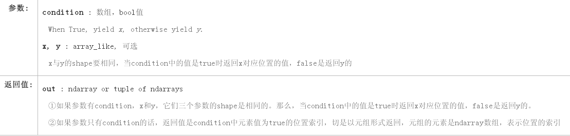
1 | np.where([[True, False], [True, True]], |
np.where作为索引:
1 | In [1]: import numpy as np |
np.where多条件索引。
1 | In [5]: a = np.arange(12).reshape(3,4) |
np.where找到all pixels of specific BGR value,代码如下:
1 | # red shape: 2x5x3 |
np.pad
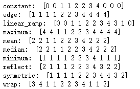
对一维数组的填充
1 | import numpy as np |
解释:
- 第一个参数是待填充数组
- 第二个参数是填充的形状,(2,3)表示前面两个,后面三个
- 第三个参数是填充的方法
填充方法:
- constant连续一样的值填充,有关于其填充值的参数。constant_values=(x, y)时前面用x填充,后面用y填充。缺参数是为0000。。。
- edge用边缘值填充
- linear_ramp边缘递减的填充方式
- maximum, mean, median, minimum分别用最大值、均值、中位数和最小值填充
- reflect, symmetric都是对称填充。前一个是关于边缘对称,后一个是关于边缘外的空气对称╮(╯▽╰)╭
- wrap用原数组后面的值填充前面,前面的值填充后面
- 也可以有其他自定义的填充方法
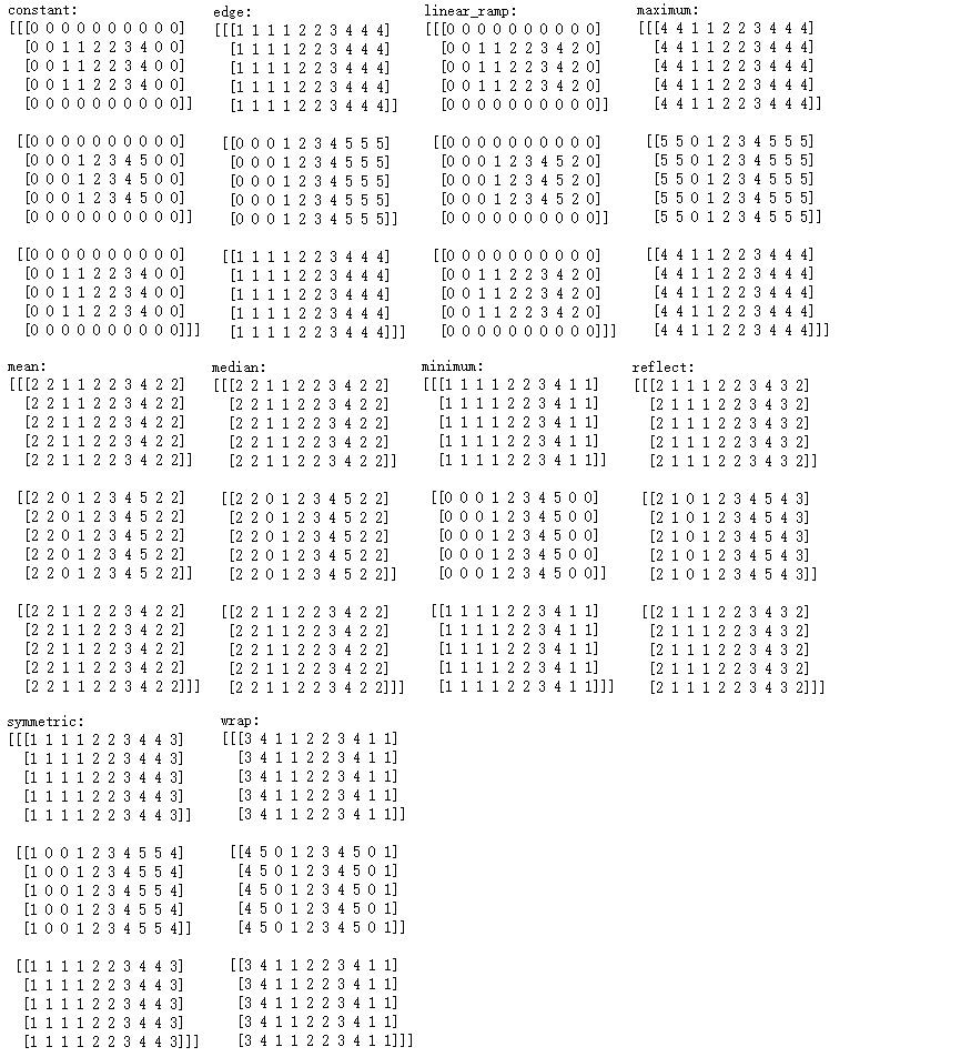
对多维数组的填充
1 | import numpy as np |
numpy、list、mat区别
1 | print a |
打印全部元素
添加下面语句即可。
1 | set_printoptions(threshold='nan') |
np.ascontiguousarray
返回连续内存空间的矩阵
1 | >>> np.ascontiguousarray(x, dtype=np.float32) |
得到矩阵最大值所在的行与列
1 | a = np.arange(6).reshape(2,3) |
参考
NumPy之四:高级索引和索引技巧
python 的numpy库中的mean()函数用法
提取numpy矩阵的上三角或下三角部分
用Numpy求逆矩阵?
python中找出numpy array数组的最值及其索引
OpenCV: setting all pixels of specific BGR value to another BGR value
np.where()多条件用法